Assume that, for some reasons, you weight a can of tuna by kitchen scale and notice that the weight is quite smaller than it should be. As you are a persistent person you keep weighting 6 more cans and the average weight is still far from what is mentioned on the label. So You probably wonder if the company is cheating and if you have found trustable evidence, no?

Notice that your evidence, the can’s average weight, is based on the sample of only 7 cans you could get your hands on. However, what you want to claim is about the average weight of the whole population of tuna cans that the company produces. Are we able to prove this fraud with such a small sample?
This problem is very common in statistics when you need to make a judgement on the population mean based on the sample mean. Such a judgement is ultimately important in practice, as the population is often not accessible or it is quite costly and difficult to do the investigation on. This is the main motivation for the t-test!
Let us first introduce some simple notations:
- n: number of samples: X1, X2, ...,Xn
- X and s: mean and standard deviation of the sample
- μ and σ: mean and standard deviation of the population
Assume that the population is normal, which means that when you repeat your experiment (on n samples) lots of times (k times), and you compute and plot the sample mean X each time, you will end up with the Gaussian (bell-shaped) distribution. The following graph is plotted with k = 20000 and for the average weight of tuna cans as 150gr.

One can prove that

This seems useful as the famous 68–95–99.7 rule tells us that there is 99.7% chance that:
So, after some simple manipulations, we get an estimate for the population mean:
which is very very likely to be true (OMG 99.7%!).
So, based on one small sample of size n we can estimate 𝝁, and what if the nominal weight on the label does not satisfy this estimate? The company is, very likely, cheating!

t-score
Things seem too good to be true, no? Note that the interesting calculation based on z-score requires having the standard deviation of the population. Do we have it? Often not!
One may wonder to replace with the sample standard deviation s. This is how we end up with the so-called t-value:

The problem is not still solved! The issue is that for z, we had z~N(0,1) based on which we found the final estimate for 𝝁; but, what can one say about t?
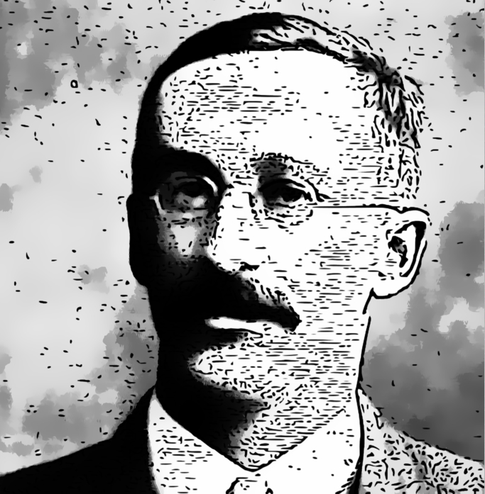
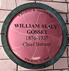
It was William Sealy Gosset, an Irish statistician working at Guinness Brewery who addressed this question. He found out that the t-score, unlike the z-score, does not follow the normal distribution but another distribution, which is what we call the t-distribution with 𝛎=n-1 degrees of freedom:

In this graph, we have plotted the normal distribution as well as t-distribution with different sample sizes or degrees of freedom:

As one can see when the size of the sample is small, the t-distribution is quite different from the normal distribution, but as the sample gets larger, the t-distribution gets closer and closer to the normal distribution. They are almost the same for samples of size more than 30.
So, the problem is solved: we know the distribution of the t-score, we can determine the region of 99.7% probability around zero, we do similar calculations as before and we obtain an estimate of the population mean using X and s.
A bit of history
Gosset published his seminal work, “The probable error of a mean” in 1908, but not under his own name! He, instead, used the pen name “Student” and this is why today we call his distribution Student’s t-distribution. This is, happily, much simpler than the name he had chosen: “frequency distribution of standard deviations of samples drawn from a normal population”!
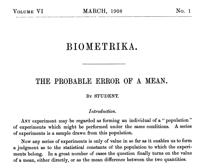
It is not crystal clear why he used a pen name and why he chose “Student”! Perhaps it was due to Guinness Brewery’s secrecy policy. Yet another interesting explanation is that the famous Karl Pearson, the editor of the journal Biometrika in which the paper was published, did not want it to be known that the paper had been written by a brewer!
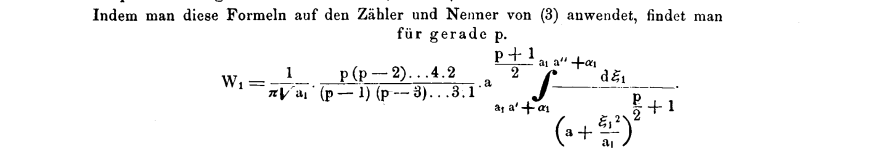
Usually, people relate the t-distribution to Gosset. However, this distribution had been discovered in Germany, around the same time that Gosset got born (1876)! Friedrich Robert Helmert, in a series of articles (1875-1876) provided correct mathematical proofs of all necessary elements in finding the t-distribution. He only needed a simple calculation to reach what Gosset reached 32 years after him; but, he was not interested! Clearly, his work was unknown to English statisticians, including Gosset, and he had to solve his problem by himself. Lacking Helmert's analytic power, Gosset based his result on two “assumptions” which later proved by another great name in statistics, Ronald Fisher!
Also in 1876, the eminent German mathematician, Jacob Lüroth, had obtained the t-distribution in his paper entitled “Vergleichung von zwei Werten des wahrschein lichen Fehlers“. His work was, however, based on some unexplained assumptions.