What is an Asymptotic Preserving (AP) scheme? A conceptual journey!

The term of Asymptotic Preserving has been coined by Shi Jin, a well-known Chinese mathematician. However, it has been rooted in USSR (as lots of other things in mathematics). In this post, I am going to review AP schemes, in a simplified language..

---

Let's right start with an example: Assume that you want to solve this simplified advection-diffusion equation: \[\nu\,u''+ u'=0\qquad \text{ over } [0,1] \quad \text{such that }\quad u(0)=0, u(1)=1,\] with two Dirichlet (fixed values) boundary conditions. One can simply confirm (believe me, it's really simple!) that the function \(u(x)=\dfrac{1-e^{-x/\nu}}{1-e^{-1/\nu}}\) satisfies this equation. If we plot this exact solution with different diffusivity constant \(\nu\), we will get this:

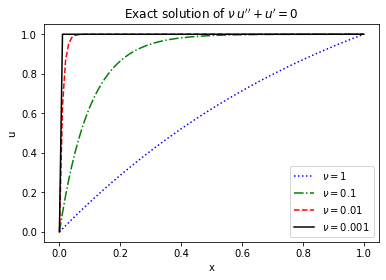As one can see, the solution develops a so-called "boundary layer" near the left boundary, which gets sharper and sharer as \(\nu\to 0\). So far so good, hein? But what happens if you want to obtain this solution numerically? This is what Il'in tried to do in 1969, in a paper titled "Differencing scheme for a differential equation with a small parameter affecting the highest derivative", and he found out that the answer is not that easy!

First, he tried a very simple finite difference discretization of the second and first-order terms, and he got the numerical solution as \(u^h_h=\dfrac{1-\left(\frac{2\nu-h}{2\nu+h}\right)^k}{1-\left(\frac{2\nu-h}{2\nu+h}\right)^N}\) which gives the following plot with \(h \approx 0.01\):

The solution does not make any sense when \(\nu\ll h\). It is not crystal clear to me the method he used here (old Soviet style paper-writing!) but one may guess that a second-order central difference for the advection term would produce a similar effect, which you can confirm in my jupyter notebook.

Investigating this issue, he then succeeded to find another discretization (probably upwind method) which provided a reasonable solution \(u^h_k=\dfrac{1-\left(\frac{\nu}{\nu+h}\right)^k}{1-\left(\frac{\nu}{\nu+h}\right)^N}\):

In summary: Depending on the discretization one uses for the each term, the numerical solution may get inaccurate (or even unstable) if \(\nu\) gets much smaller than your grid size! In other words, the solution may look good for \(ν=1\) but it is not uniformly accurate when \(ν\to 0\).

This paper, as well as a couple of others published in USSR, founded the methods that are known today as AP or Asymptotic Preserving methods. As the name implies, AP methods are defined to "preserve the asymptotic". To understand it better, consider the famous AP diagram:

\(\mathcal{M}^\varepsilon\) is the \(\varepsilon\)-dependent equation we want to solve, like the advection-diffusion example. We know that as \(\varepsilon\to 0\) (or \(\nu\) in our example) this equation will converge to its asymptotic limit \(\mathcal{M}^0\). Now, consider \(\Delta\) as the discretization parameter (like grid size \(h\) in our example). Then, the numerical deiscrete model \(\mathcal{M}^\varepsilon_\Delta\):

• Converges to the continuous equation \(\mathcal{M}^\varepsilon\), for a fixed \(\varepsilon\) when the grid gets refined \(\Delta\to 0\). 
• Converges to the numerical asymptotic solution \(\mathcal{M}^0_\Delta\), for a fixed discretization when the parameter vanishes \(\varepsilon \to 0\)

As we observed in the advection-diffusion example, the \(\mathcal{M}^\varepsilon_\Delta\to \mathcal{M}^0_\Delta\) convergence did not hold unless the grid get refined as \(\varepsilon\to 0\). This poses a big issue in practice, as refining the grid increases the computational cost of the method. Sometimes, this convergence holds, but \(\mathcal{M}^0_\Delta\) is not consistent with the continous asymptotic limit \(\mathcal{M}^0\) perhaps because of an artificial \(\mathcal{O}(1/\varepsilon)\) diffusion term which does not make the asymptotic method unstable but incosistent with the real model. One can still find lots of other interesting examples to explain AP schemes. I did a brief introduction here with another example of van der Pol system in my SlideShare: